Plotting mixture models in ggplot2
This post deals with something niche but practical - getting ggplot2 to plot multiple fitted gaussians from a model with different amplitudes. Google failed to provide the answer I was looking for - if you can’t find it with Google, it must need a blog post.
We have a couple of different projects running at the moment that need us to
think about mixture models - these are common in single molecule biophysics work
as you frequently end up with two or more populations of molecules stretched out
along a continuous variable; could be velocity, step size or something else. A
common solution to figuring out what the typical representative values are in
the mixed population is to fit multiple gaussians to the data and describe the
mean and standard deviation of each. Doing this also allows you to describe the
relative size of each population if this changes with conditions. The mixtools
package1 for R
does all this and more - it’s a fantastic resource (and the
vignette2
is really well written too).
There are already some great blog posts3 4 that go into using the
normalmixEM function to find a specified number (k) of best fit gaussians
for your data. And also some that do a far better job than this biologist is
ever going to do of explaining the Expectation-Maximization Algorithm5 that’s
at work. It’s worth noting that mixtools has a whole suite of tools for
estimating the number of gaussians in your sample (not trivial) and can deal
with non-normal distributions.
set up and getting the model
#libraries needed
library(tidyverse)
library(mixtools)

#just a plotting theme
ggplot2::theme_set(
  theme_bw() +
    theme(
      plot.title = element_text(size = 14),
      axis.title = element_text(size = 14, colour = "grey30"),
      axis.text = element_text(size = 12, colour = "grey30"),
      panel.grid = element_blank()
    )
)
First let’s simulate a data set comprised of two groups with different means and the same standard deviation, but with half the observations in one group compared to the other:
set.seed(12) #better make this reproducible
observations <- tibble(value = c(
rnorm(n = 125, mean = 0.1, sd = 0.2), #the first normal distribution
rnorm(n = 250, mean = 0.8, sd = 0.2) #this second distribution is double the size of the first
)
)
#and a quick gander...
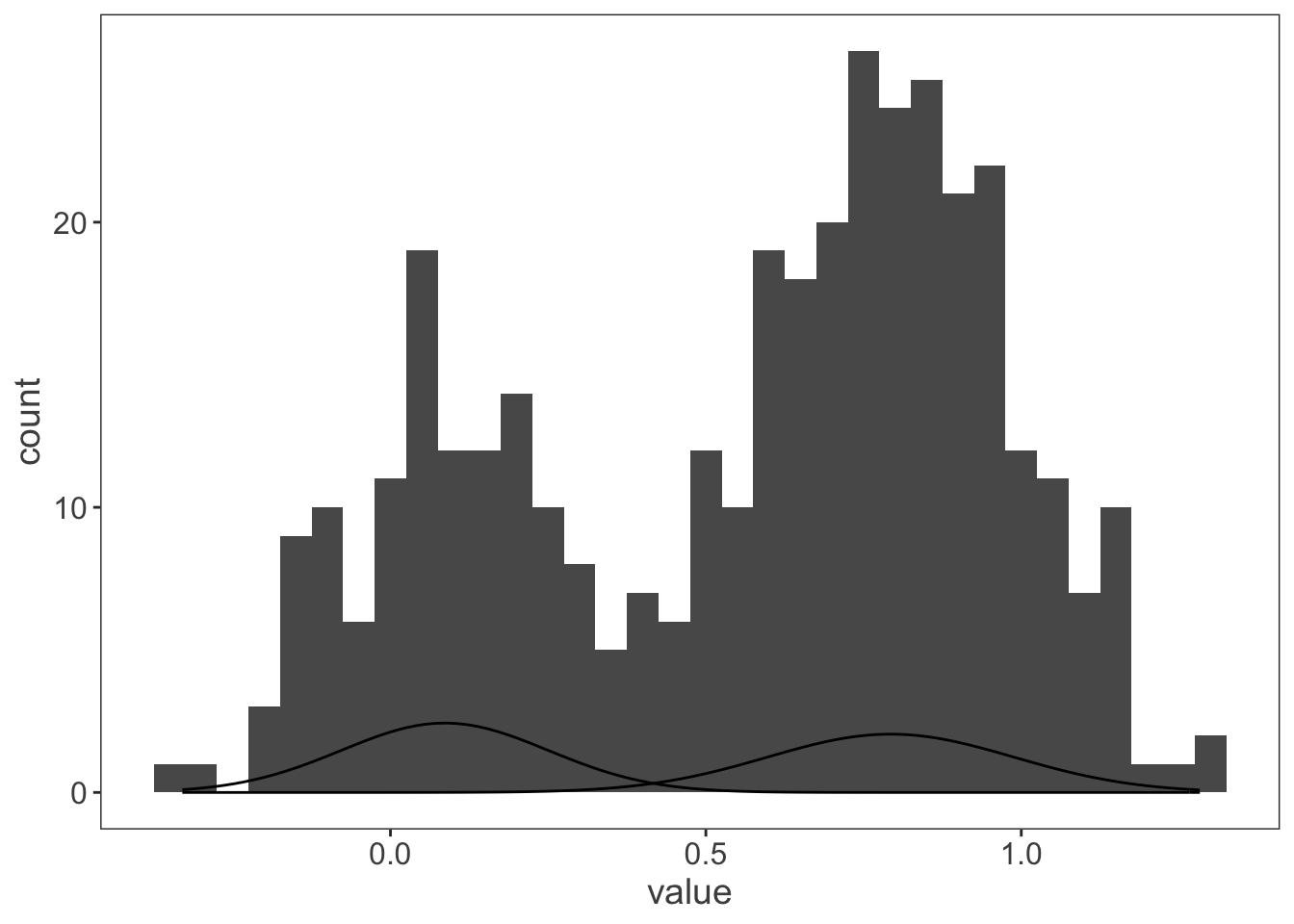
ggplot(observations, aes(x = value)) +
geom_histogram(binwidth = 0.05)
Next let’s get mixtools to figure out where it thinks those gaussians are:
my_mix <- normalmixEM(observations$value, k = 2) #telling it to find two gaussians in the observations## number of iterations= 38plot(my_mix, which = 2) #looking at the model produced with base graphics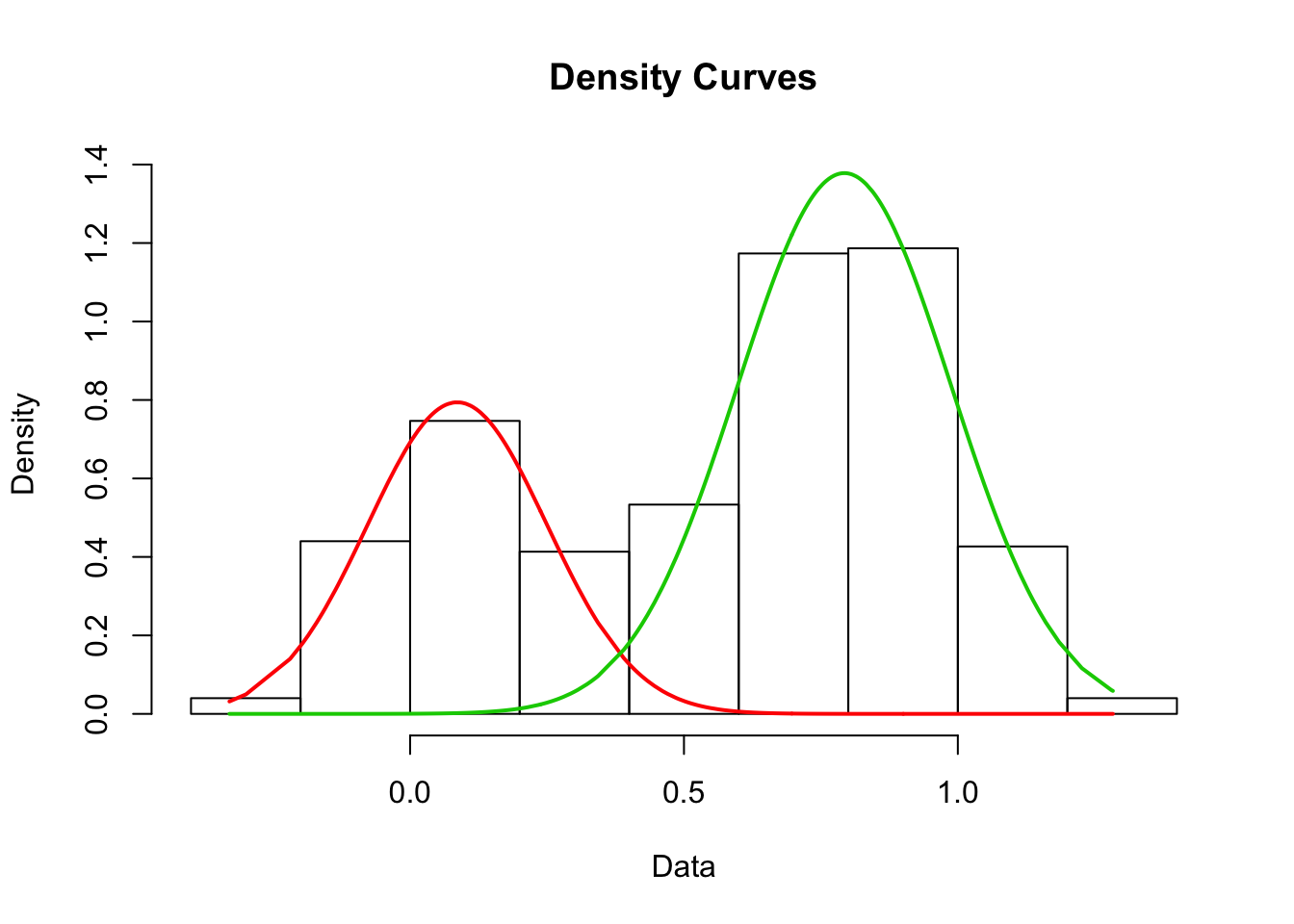
the problem
For publication ready plots we need to move over to ggplot2 rather than base
graphics (some will argue no doubt, but there’s value in making graphics as
human friendly as possible for communicating science).
normalmixEM provides a list of 9 outputs for the gaussians it calculates,
including the mean, standard deviation and amplitude:
my_mix[["mu"]] #means## [1] 0.08612553 0.79291123my_mix[["sigma"]] #standard deviations## [1] 0.1638908 0.1950395my_mix[["lambda"]] #amplitudes## [1] 0.3262176 0.6737824It’s straight forward enough to use dnorm with stat_function to plot a
gaussian line on top of a histogram. Two gaussians requires two stat_functions
- not a big deal, but if you’ve got a data set with four or five, or you want to
insert this more programmatically into an analysis script you quickly hit
problems.
ggplot(observations, aes(x = value)) +
  geom_histogram(binwidth = 0.05) +
  stat_function(fun = dnorm,
                args = list(mean = my_mix[["mu"]][[1]],
                            sd = my_mix[["sigma"]][[1]])) +
  stat_function(fun = dnorm,
                args = list(mean = my_mix[["mu"]][[2]],
                            sd = my_mix[["sigma"]][[2]]))
There’s another couple of problems immediately. The gaussians are expressed as
densities and the histogram as counts. Adding the aes y = ..density.. to the
histogram can fix this problem, but only if you want to express the data as a
density instead of event counts. More difficult, dnorm doesn’t have an
argument for the relative amplitude, so both gaussians have the same area. Three
things need fixing - plot all the gaussians in a single call, convert them to be
proportional to counts and incorporate the relative amplitude. Plotting multiple
instances of a function requires mapply - the above plot can also be made like
this:
ggplot(observations, aes(x = value)) +
  geom_histogram(binwidth = 0.05) +
  mapply(function(mean, sd) {
    stat_function(fun = dnorm, args = list(mean = mean, sd = sd))
    },
    #the argument definitions hang out down here
    mean = my_mix[["mu"]],
    sd = my_mix[["sigma"]]
  )
the solution
Scaling the gaussian density to the count number requires taking into account
the number of observations in the data set and the bin width of the histogram.
If we’re creating a function to modify dnorm then it can also incorporate the
amplitude, my_mix[["lambda"]]. I need to nest a new function with extra
arguments inside stat_function to modify dnorm.
ggplot(observations, aes(x = value)) +
  geom_histogram(binwidth = 0.05) +
  mapply(
    function(mean, sd, lambda, n, binwidth) {
      stat_function(
        fun = function(x) {
          (dnorm(x, mean = mean, sd = sd)) * n * binwidth * lambda
        }
      )
    },
    mean = my_mix[["mu"]], #mean
    sd = my_mix[["sigma"]], #standard deviation
    lambda = my_mix[["lambda"]], #amplitude
    n = length(observations$value), #sample size
    binwidth = 0.05 #binwidth used for histogram
  )
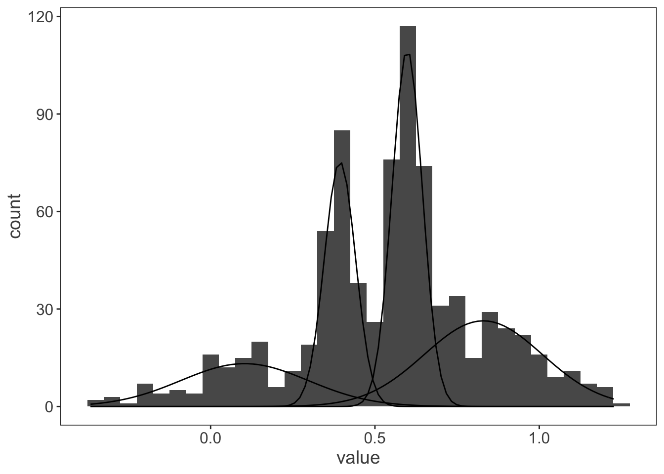
That’s more like it! And just to check it works for a more complicated data set with more than two distributions:
observations <- tibble(value = c(
  rnorm(n = 125, mean = 0.1, sd = 0.2),
  rnorm(n = 175, mean = 0.4, sd = 0.05),
  rnorm(n = 250, mean = 0.6, sd = 0.05),
  rnorm(n = 250, mean = 0.8, sd = 0.2)
  )
  )

my_mix <- normalmixEM(observations$value, k = 4)
## number of iterations= 167ggplot(observations, aes(x = value)) +
geom_histogram(binwidth = 0.05) +
mapply(function(mean, sd, lambda, n, binwidth) {
stat_function(
fun = function(x) {
(dnorm(x, mean = mean, sd = sd)) * n * binwidth * lambda
}
)
},
mean = my_mix[["mu"]],
sd = my_mix[["sigma"]],
lambda = my_mix[["lambda"]],
n = length(observations$value),
binwidth = 0.05
)
R session
devtools::session_info()## ─ Session info ──────────────────────────────────────────────────────────
## setting value
## version R version 3.6.0 (2019-04-26)
## os macOS Mojave 10.14
## system x86_64, darwin15.6.0
## ui X11
## language (EN)
## collate en_GB.UTF-8
## ctype en_GB.UTF-8
## tz Europe/London
## date 2019-06-19
##
## ─ Packages ──────────────────────────────────────────────────────────────
## package * version date lib source
## assertthat 0.2.1 2019-03-21 [1] CRAN (R 3.6.0)
## backports 1.1.4 2019-04-10 [1] CRAN (R 3.6.0)
## blogdown 0.13 2019-06-11 [1] CRAN (R 3.6.0)
## bookdown 0.11 2019-05-28 [1] CRAN (R 3.6.0)
## broom 0.5.2 2019-04-07 [1] CRAN (R 3.6.0)
## callr 3.2.0 2019-03-15 [1] CRAN (R 3.6.0)
## cellranger 1.1.0 2016-07-27 [1] CRAN (R 3.6.0)
## cli 1.1.0 2019-03-19 [1] CRAN (R 3.6.0)
## colorspace 1.4-1 2019-03-18 [1] CRAN (R 3.6.0)
## crayon 1.3.4 2017-09-16 [1] CRAN (R 3.6.0)
## desc 1.2.0 2018-05-01 [1] CRAN (R 3.6.0)
## devtools 2.0.2 2019-04-08 [1] CRAN (R 3.6.0)
## digest 0.6.19 2019-05-20 [1] CRAN (R 3.6.0)
## dplyr * 0.8.1 2019-05-14 [1] CRAN (R 3.6.0)
## evaluate 0.14 2019-05-28 [1] CRAN (R 3.6.0)
## forcats * 0.4.0 2019-02-17 [1] CRAN (R 3.6.0)
## fs 1.3.1 2019-05-06 [1] CRAN (R 3.6.0)
## generics 0.0.2 2018-11-29 [1] CRAN (R 3.6.0)
## ggplot2 * 3.1.1 2019-04-07 [1] CRAN (R 3.6.0)
## glue 1.3.1 2019-03-12 [1] CRAN (R 3.6.0)
## gtable 0.3.0 2019-03-25 [1] CRAN (R 3.6.0)
## haven 2.1.0 2019-02-19 [1] CRAN (R 3.6.0)
## hms 0.4.2 2018-03-10 [1] CRAN (R 3.6.0)
## htmltools 0.3.6 2017-04-28 [1] CRAN (R 3.6.0)
## httr 1.4.0 2018-12-11 [1] CRAN (R 3.6.0)
## jsonlite 1.6 2018-12-07 [1] CRAN (R 3.6.0)
## knitr 1.23 2019-05-18 [1] CRAN (R 3.6.0)
## labeling 0.3 2014-08-23 [1] CRAN (R 3.6.0)
## lattice 0.20-38 2018-11-04 [1] CRAN (R 3.6.0)
## lazyeval 0.2.2 2019-03-15 [1] CRAN (R 3.6.0)
## lubridate 1.7.4 2018-04-11 [1] CRAN (R 3.6.0)
## magrittr 1.5 2014-11-22 [1] CRAN (R 3.6.0)
## MASS 7.3-51.4 2019-03-31 [1] CRAN (R 3.6.0)
## Matrix 1.2-17 2019-03-22 [1] CRAN (R 3.6.0)
## memoise 1.1.0 2017-04-21 [1] CRAN (R 3.6.0)
## mixtools * 1.1.0 2017-03-10 [1] CRAN (R 3.6.0)
## modelr 0.1.4 2019-02-18 [1] CRAN (R 3.6.0)
## munsell 0.5.0 2018-06-12 [1] CRAN (R 3.6.0)
## nlme 3.1-140 2019-05-12 [1] CRAN (R 3.6.0)
## pillar 1.4.1 2019-05-28 [1] CRAN (R 3.6.0)
## pkgbuild 1.0.3 2019-03-20 [1] CRAN (R 3.6.0)
## pkgconfig 2.0.2 2018-08-16 [1] CRAN (R 3.6.0)
## pkgload 1.0.2 2018-10-29 [1] CRAN (R 3.6.0)
## plyr 1.8.4 2016-06-08 [1] CRAN (R 3.6.0)
## prettyunits 1.0.2 2015-07-13 [1] CRAN (R 3.6.0)
## processx 3.3.1 2019-05-08 [1] CRAN (R 3.6.0)
## ps 1.3.0 2018-12-21 [1] CRAN (R 3.6.0)
## purrr * 0.3.2 2019-03-15 [1] CRAN (R 3.6.0)
## R6 2.4.0 2019-02-14 [1] CRAN (R 3.6.0)
## Rcpp 1.0.1 2019-03-17 [1] CRAN (R 3.6.0)
## readr * 1.3.1 2018-12-21 [1] CRAN (R 3.6.0)
## readxl 1.3.1 2019-03-13 [1] CRAN (R 3.6.0)
## remotes 2.0.4 2019-04-10 [1] CRAN (R 3.6.0)
## rlang 0.3.4 2019-04-07 [1] CRAN (R 3.6.0)
## rmarkdown 1.13 2019-05-22 [1] CRAN (R 3.6.0)
## rprojroot 1.3-2 2018-01-03 [1] CRAN (R 3.6.0)
## rstudioapi 0.10 2019-03-19 [1] CRAN (R 3.6.0)
## rvest 0.3.4 2019-05-15 [1] CRAN (R 3.6.0)
## scales 1.0.0 2018-08-09 [1] CRAN (R 3.6.0)
## segmented 0.5-4.0 2019-05-13 [1] CRAN (R 3.6.0)
## sessioninfo 1.1.1 2018-11-05 [1] CRAN (R 3.6.0)
## stringi 1.4.3 2019-03-12 [1] CRAN (R 3.6.0)
## stringr * 1.4.0 2019-02-10 [1] CRAN (R 3.6.0)
## survival 2.44-1.1 2019-04-01 [1] CRAN (R 3.6.0)
## tibble * 2.1.3 2019-06-06 [1] CRAN (R 3.6.0)
## tidyr * 0.8.3 2019-03-01 [1] CRAN (R 3.6.0)
## tidyselect 0.2.5 2018-10-11 [1] CRAN (R 3.6.0)
## tidyverse * 1.2.1 2017-11-14 [1] CRAN (R 3.6.0)
## usethis 1.5.0 2019-04-07 [1] CRAN (R 3.6.0)
## withr 2.1.2 2018-03-15 [1] CRAN (R 3.6.0)
## xfun 0.7 2019-05-14 [1] CRAN (R 3.6.0)
## xml2 1.2.0 2018-01-24 [1] CRAN (R 3.6.0)
## yaml 2.2.0 2018-07-25 [1] CRAN (R 3.6.0)
##
## [1] /Library/Frameworks/R.framework/Versions/3.6/Resources/library
