Plotting mixture models, part 2: sum of gaussians
In the previous post I plotted multiple fit gaussians onto a data set with
ggplot2 - the final model is actually the sum of these fitted gaussians though,
so how do I plot that? This is a more tricksy problem. I know I need to nest
the mapply function inside another function, but my mind doesn’t immediately
leap to the answer - I tried to come up with something quickly, but it
inevitably failed.
My approach to fixing analysis problems like this is to break it down and build up the complexity slowly until I get something that works. Rather than working over the same code until it was right, this time I kept track of my iterations so I had something I could use to demonstrate my approach to my students.
An aside on why I think it’s important: I really want to create an environment in my lab where folks are comfortable with coding (so far it’s working!); I share Steve Royle’s view that “[computer-based methods] have now permeated mainstream […] cell biology to such an extent that any groups that want to do cell biology in the future have to adapt”. We’re wet lab scientists, and almost all my students coming in don’t have huge experience in analyzing data with a programming language. I didn’t learn R until I self-taught as a postdoc. One of the things that made it difficult to learn was when you did figure out an answer with Google and stack overflow, it was usually just presented to you - “Ta da! I’m smart look at my solution!”. This gives the impression that if you know R/python/whatever you should just know the answer - but really getting things to work requires the same sort of focus and optimizing of a protocol as bench work. You can do it in a structured way and with more experience you get better, just like bench work. For me, part of fostering the right environment to encourage people to pick up R and python and be comfortable not always getting it right, is to show how I work through some problems.
where we left off
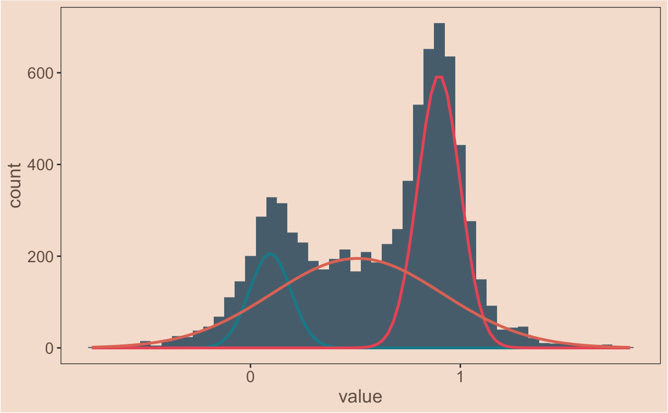
I kick off where I left off, plotting the gaussians on a simulated data set
#libraries needed
library(tidyverse)
library(mixtools)
library(ghibli) #' if I want to look less professional by having
                #' studio ghibli themed plots on my blog that's my choice, okay?

#just a plotting theme
ggplot2::theme_set(
  theme_bw() +
    theme(
      plot.background = element_rect(fill = ghibli_palettes$PonyoLight[7]),
      panel.background = element_rect(fill = ghibli_palettes$PonyoLight[7]),
      plot.title = element_text(size = 14),
      axis.title = element_text(size = 14, colour = ghibli_palettes$PonyoDark[7]),
      axis.text = element_text(size = 12, colour = ghibli_palettes$PonyoDark[7]),
      panel.grid = element_blank()
    )
)

#simulate a dataset
set.seed(12) #better make this reproducible
observations <- tibble(value = c(
  rnorm(n = 1000, mean = 0.1, sd = 0.1),
  rnorm(n = 4000, mean = 0.5, sd = 0.4),
  rnorm(n = 3000, mean = 0.9, sd = 0.1)
  )
  )

#model the dataset with multiple gaussians
my_mix <- normalmixEM(observations$value, k = 3)
## number of iterations= 374#plot the data and the model
ggplot(observations, aes(x = value)) +
geom_histogram(binwidth = 0.05, fill = ghibli_palettes$PonyoMedium[2]) +
mapply(function(mean, sd, lambda, n, binwidth, colour) {
stat_function(
fun = function(x) {
(dnorm(x, mean = mean, sd = sd)) * n * binwidth * lambda
},
colour = colour, #this is just to make it pretty
size = 1
)
},
mean = my_mix[["mu"]],
sd = my_mix[["sigma"]],
lambda = my_mix[["lambda"]],
n = length(observations$value),
binwidth = 0.05,
colour = c(ghibli_palettes$PonyoMedium[3],
ghibli_palettes$PonyoMedium[4],
ghibli_palettes$PonyoMedium[5])
)
where do I start?
[warning - this really does go at a snails pace, skip to the end if you want the finished function]
Define the problem. I know what I want to do - at each point along x I want to
sum the individual guassians together to get the final model. I take this pretty
literally and start there. To make my life simpler while I focus on the problem,
I move out of plotting in ggplot for the time being and focus on the numbers.
The first thing I do is make the dnorm modification inside mapply into a
stand alone function so I can call it more easily.
#my function
proportional_gauss <- function(x, mean, sd, lambda, n, binwidth) {
        (dnorm(x, mean = mean, sd = sd)) * n * binwidth * lambda
        }
#generate a vector of x values to work with
x_values <- seq(from = -1, to = 2, length.out = 1000)I’ll make a new vector which should be the y values at any given x value for the first gaussian function from my model and then check it quickly:
model_1 <- proportional_gauss(
  x = x_values,
  mean = my_mix[["mu"]][[1]],
  sd = my_mix[["sigma"]][[1]],
  lambda = my_mix[["lambda"]][[1]],
  n = length(observations$value),
  binwidth = 0.05
)

plot(model_1)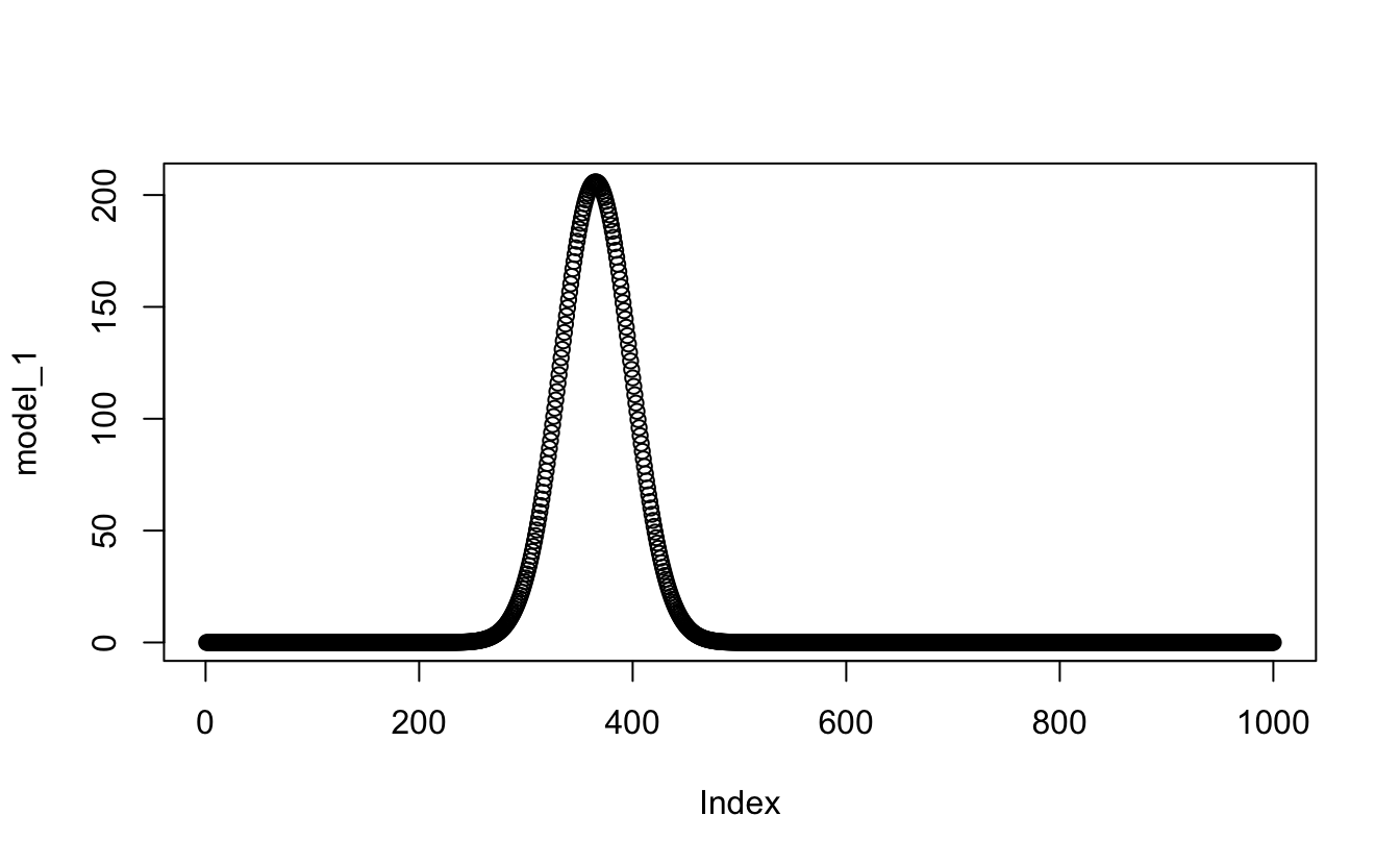
Great - that worked. I’ll make the other two then assemble them all into one
table (tibble). With dplyr I’ll add a column with mutate to have the sum of
all the models, then quickly check if this give me the data I’m after.
model_2 <- proportional_gauss(
x = x_values,
mean = my_mix[["mu"]][[2]],
sd = my_mix[["sigma"]][[2]],
lambda = my_mix[["lambda"]][[2]],
n = length(observations$value),
binwidth = 0.05
)
model_3 <- proportional_gauss(
x = x_values,
mean = my_mix[["mu"]][[3]],
sd = my_mix[["sigma"]][[3]],
lambda = my_mix[["lambda"]][[3]],
n = length(observations$value),
binwidth = 0.05
)
all_models <- tibble(x_values = x_values,
first = model_1,
second = model_2,
third = model_3) %>%
mutate(., sum = sum(first, second, third))
plot(all_models$sum) #checking the product of the data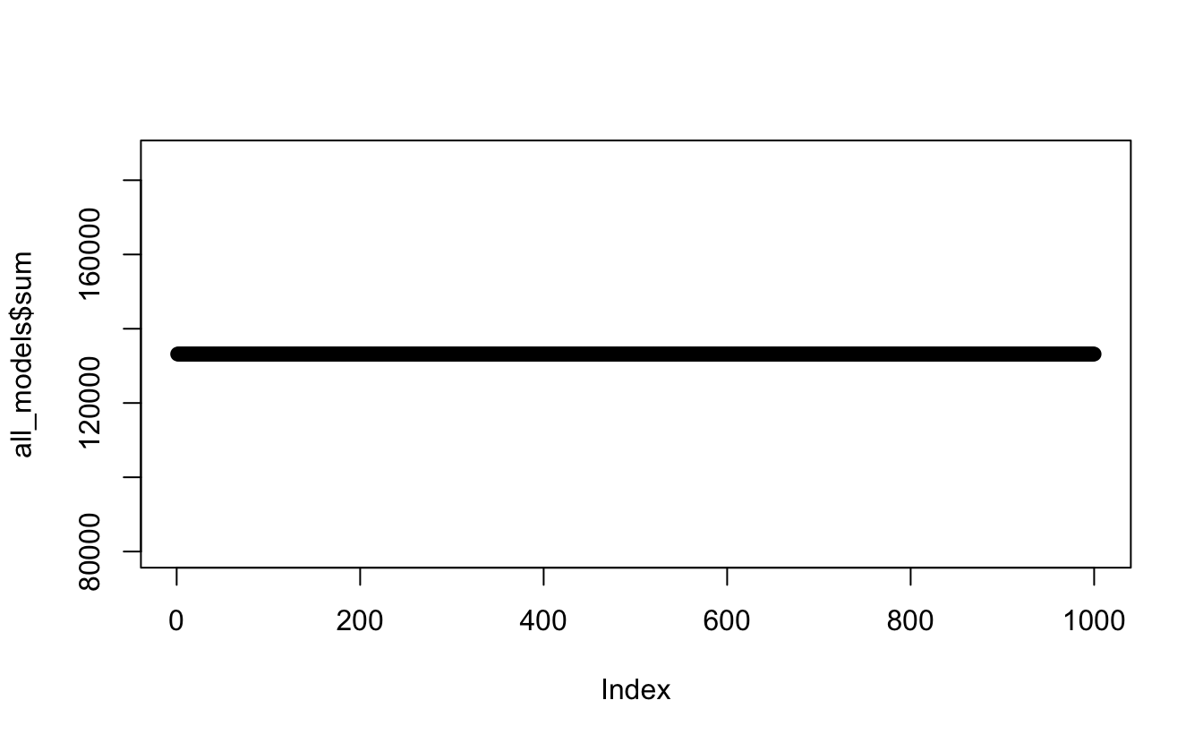 Eeeer nope… definitely not what I was hoping for. Using the
 sum function like this
has literally just summed the whole lot together, rather than at each x point.
Try again…
#this time I'll manually add the columns together

all_models <- tibble(
  x_values = x_values,
  first = model_1,
  second = model_2,
  third = model_3) %>%
  mutate(., sum = (first + second + third))

plot(all_models$sum) #checking the product of the data
Okay - Better. Seems relatively simple. But I don’t want to manually call
each model, I want to have a function call all the relevant models at once. I
Google a bit and then read the apply help file for the thousandth time and try this:
test_sum <- apply(all_models[, 2:4], 1, sum) #row sums using apply across the 2nd to fourth columns
plot(test_sum)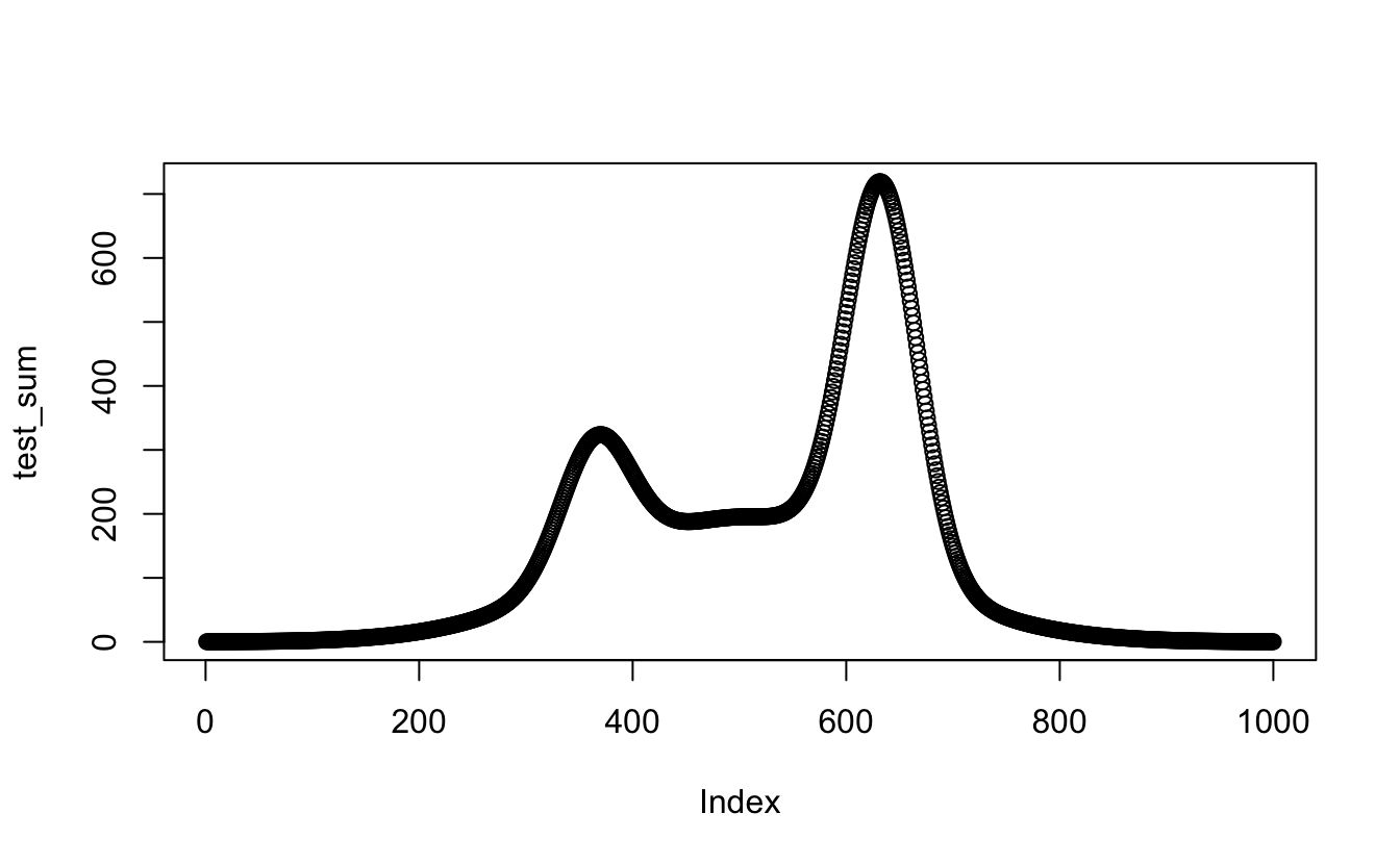
Sweet! that totally worked. Okay, now do it in the table -
#replacing the manual sum with the apply function
all_models <- tibble(
  x_values = x_values,
  first = model_1,
  second = model_2,
  third = model_3) %>%
  mutate(., sum = apply(all_models[, 2:4], 1, sum))

plot(all_models$sum)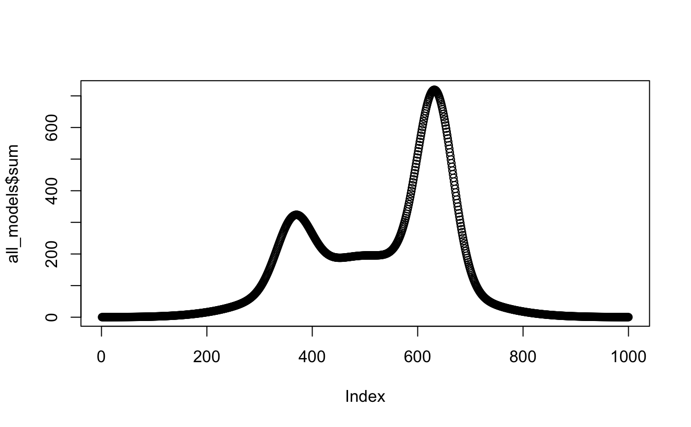
Get in! okay, next task - change the absolute references to columns, all_models[, 2:4], to relative ones with ncol():
#making the apply function in mutate generic
all_models <- tibble(
  x_values = x_values,
  first = model_1,
  second = model_2,
  third = model_3) %>%
  mutate(., sum = apply(.[, 2:ncol(.)], 1, sum))

plot(all_models$sum)
#It still works, and overlaying this manual data on the histrogram confirms it:
ggplot(observations, aes(x = value)) +
  geom_histogram(binwidth = 0.05, aes(y = ..count..),
                 fill = ghibli_palettes$PonyoMedium[2]) +
  geom_line(data = all_models, aes(x = x_values, y = sum),
            colour = ghibli_palettes$PonyoMedium[5], size = 1)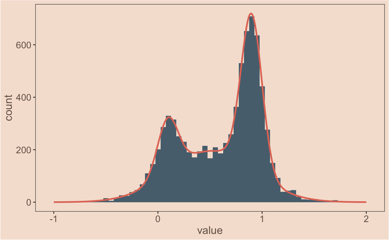
Is it possible to nest the whole function inside ggplot or is that asking for
trouble? I can only try. First I’ll nest my proportional_gauss function inside
mapply pretty much the same as I did before when I was plotting.
#this should do the same thing as before...
test <- mapply(
  proportional_gauss,
  x = x_values,
  MoreArgs = list(
    mean = my_mix[["mu"]],
    sd = my_mix[["sigma"]],
    lambda = my_mix[["lambda"]],
    n = length(observations$value),
    binwidth = 0.05
    )
  )
When I use the function on the vector x_values, I can see the product test
becomes a matrix in my environment. The model data is along the row instead of down the
column. You can see this by using the row selector, [row_number, column_number], to plot the data:
#we've got a matrix, so the data is along the row instead of down the column
plot(test[1,])
So now I need to check that apply will still work and change the MARGIN command from 1 to 2:
test2 <- apply(test, 2, sum) #which means using apply with MARGIN set to 2 not 1 to sum across the guassians
plot(test2)
#And putting it all together...
test3 <- apply(mapply(proportional_gauss,
    x = x_values,
    MoreArgs = list(
      mean = my_mix[["mu"]],
      sd = my_mix[["sigma"]],
      lambda = my_mix[["lambda"]],
      n = length(observations$value),
      binwidth = 0.05
      )
    ),
  2, sum
  )
#I guess I should plot this one too, just to be sure...

plot(test3)
Amazeballs! Happy with that. Okay, one last step; nest the proportional_gauss()
function inside a new proportional_gauss_sum() function, so I can use that inside
stat_function(). I’ll test it outside ggplot first:
proportional_gauss_sum <- function(x, mean, sd, lambda, n, binwidth) {
  apply(mapply(proportional_gauss,
                      x = x,
                      MoreArgs = list( mean, sd, lambda, n, binwidth)
                      ),
               2, sum)
}

test4 <- proportional_gauss_sum(
  x = x_values,
  mean = my_mix[["mu"]],
  sd = my_mix[["sigma"]],
  lambda = my_mix[["lambda"]],
  n = length(observations$value),
  binwidth = 0.05
)

plot(test4)
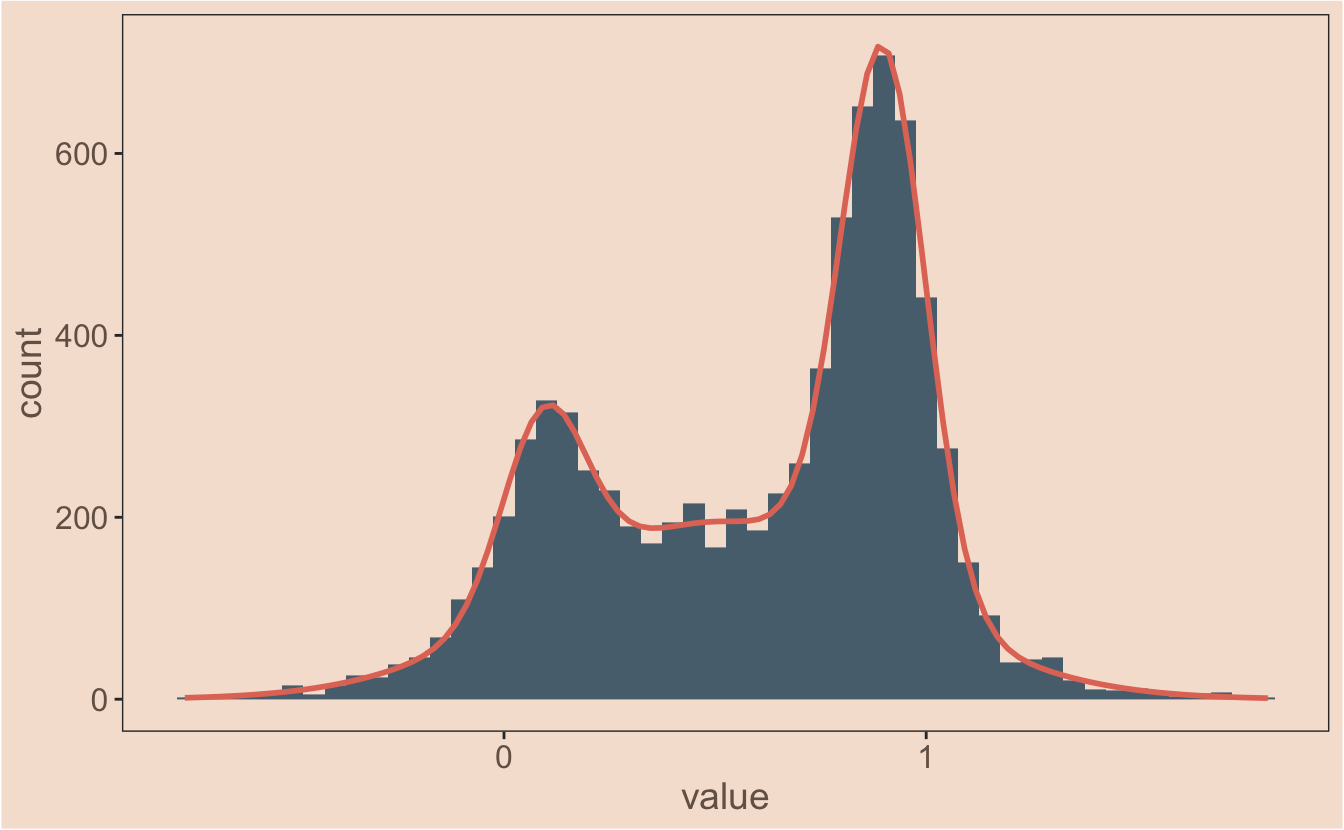
Okay - that means I’m ready for the final reveal. Ta da!
proportional_gauss <- function(x, mean, sd, lambda, n, binwidth) {
        (dnorm(x, mean = mean, sd = sd)) * n * binwidth * lambda
}


proportional_gauss_sum <- function(x, mean, sd, lambda, n, binwidth) {
  apply(mapply(proportional_gauss,
               x = x,
               MoreArgs = list( mean, sd, lambda, n, binwidth)
               ),
        2, sum)
}

ggplot(observations, aes(x = value)) +
  geom_histogram(binwidth = 0.05, fill = ghibli_palettes$PonyoMedium[2]) +
  stat_function(
    fun = proportional_gauss_sum,
    args = list(
      mean = my_mix[["mu"]],
      sd = my_mix[["sigma"]],
      lambda = my_mix[["lambda"]],
      n = length(observations$value),
      binwidth = 0.05
    ),
    colour = ghibli_palettes$PonyoMedium[5], size = 1
  )
a few comments on the process
Just as there’s more than one way to do a western blot, there’s more than one way to work through a bump in analysis. Putting all the models into a table/tibble in the begining was a bit of a wrong turn - it didn’t really help get to the solution. I ended up there because I use dplyr a lot and it’s where I’m comfortable. I do tend to plot a lot though, for me it’s the easiest way to get a sense of the shape of the data and whether I’m on the right track. I’m happy to make lot’s of incremental changes when I’m less familiar with the functions I’m using - it’s easier to keep a handle on what’s going on.
R session
devtools::session_info()## ─ Session info ──────────────────────────────────────────────────────────
## setting value
## version R version 3.6.0 (2019-04-26)
## os macOS Mojave 10.14
## system x86_64, darwin15.6.0
## ui X11
## language (EN)
## collate en_GB.UTF-8
## ctype en_GB.UTF-8
## tz Europe/London
## date 2019-06-19
##
## ─ Packages ──────────────────────────────────────────────────────────────
## package * version date lib source
## assertthat 0.2.1 2019-03-21 [1] CRAN (R 3.6.0)
## backports 1.1.4 2019-04-10 [1] CRAN (R 3.6.0)
## blogdown 0.13 2019-06-11 [1] CRAN (R 3.6.0)
## bookdown 0.11 2019-05-28 [1] CRAN (R 3.6.0)
## broom 0.5.2 2019-04-07 [1] CRAN (R 3.6.0)
## callr 3.2.0 2019-03-15 [1] CRAN (R 3.6.0)
## cellranger 1.1.0 2016-07-27 [1] CRAN (R 3.6.0)
## cli 1.1.0 2019-03-19 [1] CRAN (R 3.6.0)
## colorspace 1.4-1 2019-03-18 [1] CRAN (R 3.6.0)
## crayon 1.3.4 2017-09-16 [1] CRAN (R 3.6.0)
## desc 1.2.0 2018-05-01 [1] CRAN (R 3.6.0)
## devtools 2.0.2 2019-04-08 [1] CRAN (R 3.6.0)
## digest 0.6.19 2019-05-20 [1] CRAN (R 3.6.0)
## dplyr * 0.8.1 2019-05-14 [1] CRAN (R 3.6.0)
## evaluate 0.14 2019-05-28 [1] CRAN (R 3.6.0)
## forcats * 0.4.0 2019-02-17 [1] CRAN (R 3.6.0)
## fs 1.3.1 2019-05-06 [1] CRAN (R 3.6.0)
## generics 0.0.2 2018-11-29 [1] CRAN (R 3.6.0)
## ggplot2 * 3.1.1 2019-04-07 [1] CRAN (R 3.6.0)
## ghibli * 0.2.0 2019-03-21 [1] CRAN (R 3.6.0)
## glue 1.3.1 2019-03-12 [1] CRAN (R 3.6.0)
## gtable 0.3.0 2019-03-25 [1] CRAN (R 3.6.0)
## haven 2.1.0 2019-02-19 [1] CRAN (R 3.6.0)
## hms 0.4.2 2018-03-10 [1] CRAN (R 3.6.0)
## htmltools 0.3.6 2017-04-28 [1] CRAN (R 3.6.0)
## httr 1.4.0 2018-12-11 [1] CRAN (R 3.6.0)
## jsonlite 1.6 2018-12-07 [1] CRAN (R 3.6.0)
## knitr 1.23 2019-05-18 [1] CRAN (R 3.6.0)
## labeling 0.3 2014-08-23 [1] CRAN (R 3.6.0)
## lattice 0.20-38 2018-11-04 [1] CRAN (R 3.6.0)
## lazyeval 0.2.2 2019-03-15 [1] CRAN (R 3.6.0)
## lubridate 1.7.4 2018-04-11 [1] CRAN (R 3.6.0)
## magrittr 1.5 2014-11-22 [1] CRAN (R 3.6.0)
## MASS 7.3-51.4 2019-03-31 [1] CRAN (R 3.6.0)
## Matrix 1.2-17 2019-03-22 [1] CRAN (R 3.6.0)
## memoise 1.1.0 2017-04-21 [1] CRAN (R 3.6.0)
## mixtools * 1.1.0 2017-03-10 [1] CRAN (R 3.6.0)
## modelr 0.1.4 2019-02-18 [1] CRAN (R 3.6.0)
## munsell 0.5.0 2018-06-12 [1] CRAN (R 3.6.0)
## nlme 3.1-140 2019-05-12 [1] CRAN (R 3.6.0)
## pillar 1.4.1 2019-05-28 [1] CRAN (R 3.6.0)
## pkgbuild 1.0.3 2019-03-20 [1] CRAN (R 3.6.0)
## pkgconfig 2.0.2 2018-08-16 [1] CRAN (R 3.6.0)
## pkgload 1.0.2 2018-10-29 [1] CRAN (R 3.6.0)
## plyr 1.8.4 2016-06-08 [1] CRAN (R 3.6.0)
## prettyunits 1.0.2 2015-07-13 [1] CRAN (R 3.6.0)
## processx 3.3.1 2019-05-08 [1] CRAN (R 3.6.0)
## ps 1.3.0 2018-12-21 [1] CRAN (R 3.6.0)
## purrr * 0.3.2 2019-03-15 [1] CRAN (R 3.6.0)
## R6 2.4.0 2019-02-14 [1] CRAN (R 3.6.0)
## Rcpp 1.0.1 2019-03-17 [1] CRAN (R 3.6.0)
## readr * 1.3.1 2018-12-21 [1] CRAN (R 3.6.0)
## readxl 1.3.1 2019-03-13 [1] CRAN (R 3.6.0)
## remotes 2.0.4 2019-04-10 [1] CRAN (R 3.6.0)
## rlang 0.3.4 2019-04-07 [1] CRAN (R 3.6.0)
## rmarkdown 1.13 2019-05-22 [1] CRAN (R 3.6.0)
## rprojroot 1.3-2 2018-01-03 [1] CRAN (R 3.6.0)
## rstudioapi 0.10 2019-03-19 [1] CRAN (R 3.6.0)
## rvest 0.3.4 2019-05-15 [1] CRAN (R 3.6.0)
## scales 1.0.0 2018-08-09 [1] CRAN (R 3.6.0)
## segmented 0.5-4.0 2019-05-13 [1] CRAN (R 3.6.0)
## sessioninfo 1.1.1 2018-11-05 [1] CRAN (R 3.6.0)
## stringi 1.4.3 2019-03-12 [1] CRAN (R 3.6.0)
## stringr * 1.4.0 2019-02-10 [1] CRAN (R 3.6.0)
## survival 2.44-1.1 2019-04-01 [1] CRAN (R 3.6.0)
## tibble * 2.1.3 2019-06-06 [1] CRAN (R 3.6.0)
## tidyr * 0.8.3 2019-03-01 [1] CRAN (R 3.6.0)
## tidyselect 0.2.5 2018-10-11 [1] CRAN (R 3.6.0)
## tidyverse * 1.2.1 2017-11-14 [1] CRAN (R 3.6.0)
## usethis 1.5.0 2019-04-07 [1] CRAN (R 3.6.0)
## withr 2.1.2 2018-03-15 [1] CRAN (R 3.6.0)
## xfun 0.7 2019-05-14 [1] CRAN (R 3.6.0)
## xml2 1.2.0 2018-01-24 [1] CRAN (R 3.6.0)
## yaml 2.2.0 2018-07-25 [1] CRAN (R 3.6.0)
##
## [1] /Library/Frameworks/R.framework/Versions/3.6/Resources/library
